This is a little side project I have been working on for the last couple of months. Given the popularity of League of Legends as an eSport, I wanted to see if I can use some machine learning models to predict matches between professional teams. This kind of predictive analytics for sports is very common and there have been many different approaches to the problem.
Data
All of the data that I am using has been kindly provided by Tim Sevenhuysen on his website Oracle’s Elixir. I am using the Match Data from 2016 – 2018 for the project. This match data contains match statistics for players and teams from the majority of the professional leagues. Unfortunately, there isn’t a lot of data for LPL (China) because they do not make their data as accessible as other leagues. As a result, I will be excluding LPL matches from this analysis.
There are 83 features for 2016, 99 for 2017, and 105 for 2018. As the years go on, there are more and more features that are collected. I will only be using the 64 features that are the same across all 3 years:
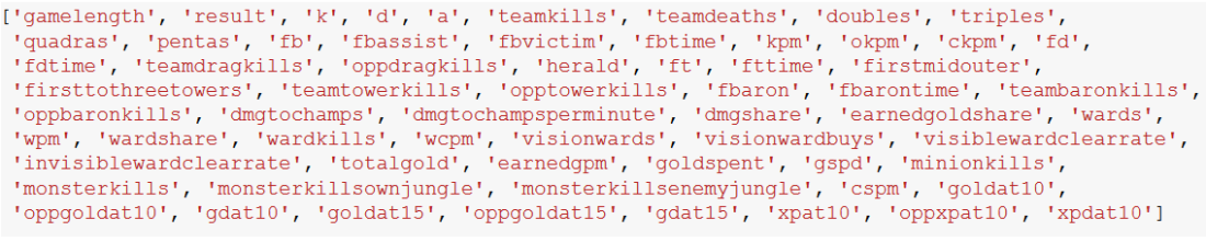
The definitions for what these features mean can be found on the data dictionary on Oracle’s Elixir. The types of stats or features that I will be using can be categorized as action/kill participation, objective control, vision control, and gold/xp generation.
For each match, I will generate features (weighted performance metrics of each player up until that match) and use the blue side (i.e. the team starting on the bottom side of the map) victory as a label (1 if blue team won, 0 if red team won). For each role on a team (Top, Jungle, Middle, ADC, and Support), I will generate weighted stats of the player in that role. So for one match, I will have 64 features per player and with 10 players that will be 640 features total. Fortunately, I have 3455 matches to work with so I will avoid the curse of dimensionality.
Methodology
My approach to this project is a simple one: given two teams with 5 players each and performance metrics for each player, can I predict which team will win? I initially considered using team based metrics instead of player based metrics but decided to go with players since the skills and performance of particular players is usually key to victory for most teams.
Time Weighted Averages
One question that immediately arises is how does one determine the performance of a player? I can use the lifetime stats of each player but that might not reflect how well a player is performing currently: a player that was dominating two years ago might not be so good this year. I decided to calculate metrics for each player based on how long ago the particular matches were. For example, if a player has played only two matches, one being yesterday and the other being a few months ago, that player’s performance for the match played a few months ago would be discounted by some factor proportional to how long ago it was. Instead of averaging his performance equally, the most recent match would have more weight. So for each match, I will generate the time weighted averages of the 64 features above for each player for all matches up until that point. I applied a weight of .05 to the earliest match and a weight of 1 to the most recent match. Additionally, stats from each passing year are discounted by 2^(t) where t is number of years passed. For example, when generating features to use in 2018, matches in 2016 will be discounted by a factor of 2^2 or 4. I added the discounting because player performances can change dramatically from year to year. So a player’s performance in a match two years ago should have a lot less impact than a match played this year in predicting how well that player will perform in a future match.
Feature Generation and Updating Stats
To start with, I used the 2016 matches to generate weighted averages of all 64 features for every unique player. These averages are the starting point for my feature generation. For every match after 2016, I would find which players were playing on each side (Blue or Red), their roles (Top, Jungle, Middle, ADC, Support), and use the weighted stats up until that point to generate features for each 10 players (64 features x 10 players = 640 final features). Afterward, I update each player’s weighted stats with how they preformed in that game. Thus for every new game, I generate features for prediction and then update each player’s stats.
New Players
One common issue that arises when using player performance to predict matches is that there are many new players for whom there is no data. This is particularly true for the data that I have since the data from the earlier years covers less leagues and thus has less players. In 2017, there were 305 unique players out of 654 that were not in the 2016 match data but that went down to 82 unique players out of 380 in 2018. To deal with this, I will use the average of all players in the year that match to fill the missing values for new players.
Model
I tried a few different models (Logit, Random Forest, Adaboost) before settling on xgboost mostly because it was fast and had a better performance than the other algorithms. Briefly, xgboost is an ensemble method that uses gradient boosting to iteratively fit weak learners that correct the errors of previous learners. Xgboost uses a decision tree as the base learner. It has many hyper-parameters to but I will only be tuning “max_depth” (maximum depth of tree), “n_estimators” (number of models in the ensemble), “learning_rate”, “colsample_bytree” (fraction of features to randomly select for each tree), “subsample” (fraction of samples to select to select for a tree). I believe one can use sklearn’s grid search functionality to tune the hyper-parameters but because xgboost was so fast, I just tried a bunch of different parameters manually until I got a combination that maximized accuracy on the testing set.
Results
Model Performance
To evaluate the performance of my model, I first divided the matches into a training (70%) and testing (30%) set. The naive accuracy (largest class) is ~55% (i.e 55% of all matches are won by the blue side team) – this is the “blue side advantage” that League analysts often talk about. Blue side teams get their first pick of champions so they often get a team composition they want whereas Red side teams only have the opportunity to counter-pick.
I performed 5 fold cross-validation on the training set using xgboost. The model achieved a mean of ~63% accuracy during cross validation with a standard deviation of ~1.3%. Afterward, I trained the model on the entire training set and evaluated accuracy on the both the training and testing set. The model achieved an accuracy of ~78% on the training set and an accuracy of ~65% on the testing set. So the model does around ~10% better than the naive accuracy.
I then subsampled my dataset to see if the performance of the model changes with sample size:
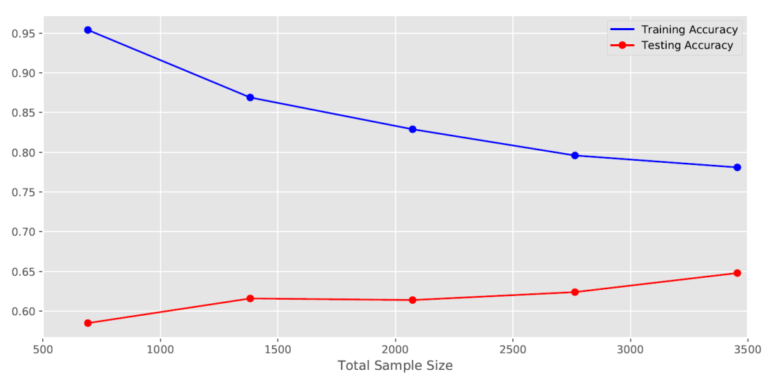
With a larger sample, the accuracy of the model tends to increase, although the increase is not that large. This may suggest that if I had more matches than I have now, the model might do even better. The model also overfits slightly as seen in the difference between the training and testing accuracy. I’m not too concerned about this since the testing accuracy is still moderately better than the naive accuracy.
I also split the data by leagues and evaluated its performance for each league separately:
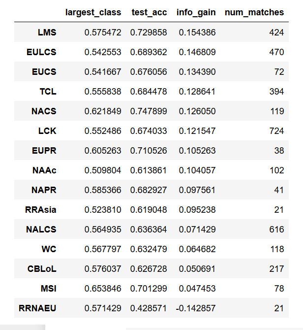
In the table above, “largest_class” is the naive accuracy (blue or red side win rate, depending on which is larger – it’s usually blue side), “test_acc” refers to the accuracy of the model in predicting matches in that region, “info_gain” refers to how well the model performs over the naive accuracy (difference between “test_acc” and “largest_class”), and “num_matches” shows the total number of matches that come from that league. For almost all regions, the model performs better than random. The one exception is “RRNAEU”, which is the Rift Rivals event for North America vs European teams. Given the low number of matches in this event (21), this might not be very important. It’s encouraging that the model achieves > 70% accuracy for some leagues as this puts it on par with some of the betting market odds (to be discussed later).
Predictive Features
Additionally, I examined the top 10 predictive features in the model. Since the final model is a collection of trees, we can pick out the features that were used to create the most informative splits. Fortunately, the python implementation of xgboost does this automatically.
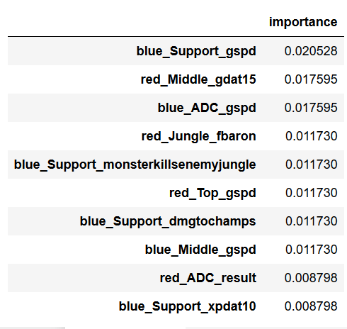
Looking at the top 10 predictive features, it seems that the performance of blue side bottom lane players (ADC and Support) seems to be the most crucial in predicting the outcome of a match. The ADC is often the key damage dealer in a team and the Support often protects and enables the ADC to farm up safely and to continuously dish out damage in team fights. It’s no surprise that the performance of the players in these two roles is important in predicting the outcome of a match. What is surprising is how often the Support role shows up in this list. Generally, Supports usually help out their other team members, particularly the ADC, and they usually don’t get a lot of gold or kills. So it’s interesting that 4 of the top 10 predictive features are some measure of the Support player’s performance.
Additionally, “gspd” (Gold Spent Percentage Difference – the percent difference between gold spent between the teams) shows up 4 times, suggesting that this may also be crucial. GSPD is a measure of how close a match was – if the GSPD between two teams was low at the end of a match, then it means they had spent equal amounts of gold by the time the game ended – indicating a close game. If the GSPD is high, then one team dominated the other, acquiring and spending more gold in the process. It seems reasonable that a team with players that consistently dominate their opponents in previous matches will be more favored to win against a team that breaks even or goes negative in GSPD.
Comparison to historical betting market odds
Next, I wanted to see how well the model compares against the public consensus as defined as historical betting market odds. For a few of the leagues, I went to the eSports section of Odds Portal and compared how often the favored team actually won vs how accurate my model was:

In general, the betting markets outperform my model quite handily. On average, the betting markets are ~75% accurate, while my model usually performs in the mid to high 60s. This probably means that there are other factors that help League of Legends analysts make better predictions. From my experience watching League matches, I would hypothesize that seeing how well a team works together to execute a win condition can help analysts compare two teams and make more accurate predictions. However, I don’t really have the data to make such an inference; the data I have is mostly limited end of match stats which can obscure how well the players worked together. For example, knowing how often the support and jungler invade to put down vision in the enemy jungle, or how the jungler starts out farming so he can end up in a certain area of the map in order to gank or counter-jungle might help my model perform better. However, it is not clear if this kind of data is available.
Conclusion and Future directions
In summary, I used a time weighted averages for players to generate role specific features for League of Legends matches in 2017 and 2018. I then used a python implementation of xgboost to perform training, cross-validation, and testing on my data. The model achieves around 65% accuracy on the testing set. Given that testing accuracy seems to increase with number of samples, the model might perform better in the future as more matches are added. Although the model performs better than random, it does not beat the accuracy of betting market odds.
Moving forward, I might try to design features that measure how well players within a team work well together. I will also look for ways to supplement my data with more informative features.
